14 Time series
14.1 Main R packages to work with time series
- astsa
- forecast
- stat
- TSA
- FitAR
- FitARMA
- MTS
- zoo
- its
- tseries
- fBasics
- …
14.2 Introduction
A time series is a collection of random variables \((X)_{t \in T}\) indexed by time i.e., \[X_1, X_2, \ldots, X_{t-1}, X_t,\] where \(T\) is a set.
14.3 Examples of time series
> x <- round(rnorm(12), 2)
>
> ts1 <- ts(x, start = 2000, frequency = 1)
> ts1
## Time Series:
## Start = 2000
## End = 2011
## Frequency = 1
## [1] 0.40 -0.61 0.34 -1.13 1.43 1.98 -0.37 -1.04 0.57 -0.14 2.40 -0.0414.4 Plotting time series
> # univariate time series
> ts4 <- ts(rnorm(100, 1, 0.25), start = 1900, frequency = 1)
> plot(ts4)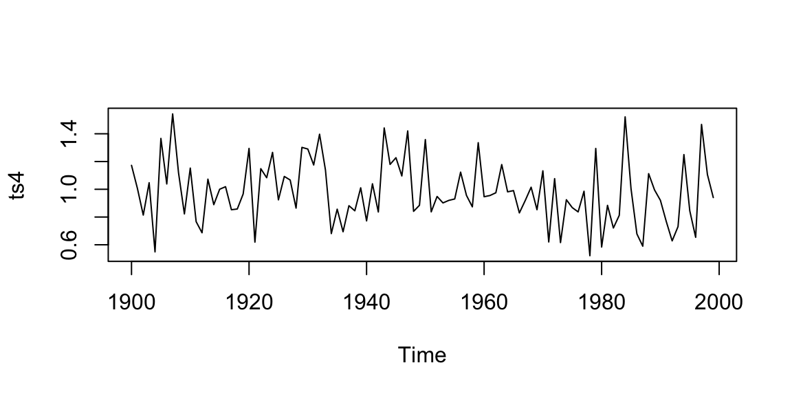
> # multivariate time series
> Mat.ts <- matrix(rnorm(200), 100, 2)
> colnames(Mat.ts) <- c("GDP", "Inflation")
> ts5 <- ts(Mat.ts, start = 1900, frequency = 1)
> plot(ts5, main = "Gross domestic product and Inflation")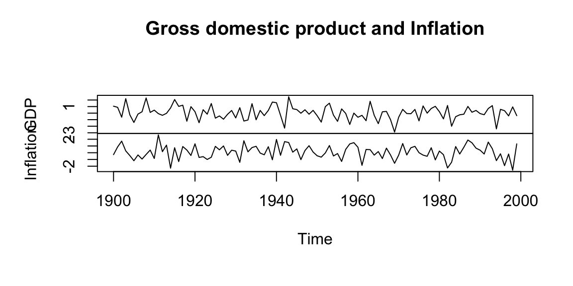
> plot(ts5, plot.type = "single", col = c("orange", "blue"), lty = c(1, 2))
> legend("bottomright", legend = colnames(Mat.ts), col = c("orange", "blue"), lty = c(1,
+     2), cex = 0.5)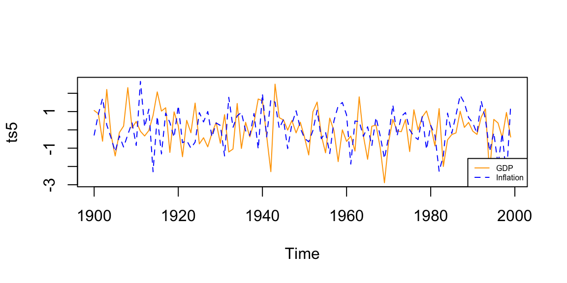
14.5 Useful functions
14.5.3 cbind: binding time series
> x1 <- round(rnorm(6), 1)
> ts7 <- ts(x1, freq = 12, start = 1959)
> ts7
##       Jan  Feb  Mar  Apr  May  Jun
## 1959 -1.2  0.0  0.1 -0.1 -0.2  1.8
>
> x2 <- round(rnorm(5), 1)
> ts8 <- ts(x2, freq = 12, start = c(1959, 3))
> ts8
##       Mar  Apr  May  Jun  Jul
## 1959  0.8  1.1 -0.9  0.2  1.2
>
> cbind(ts7, ts8)
##           ts7  ts8
## Jan 1959 -1.2   NA
## Feb 1959  0.0   NA
## Mar 1959  0.1  0.8
## Apr 1959 -0.1  1.1
## May 1959 -0.2 -0.9
## Jun 1959  1.8  0.2
## Jul 1959   NA  1.2
14.5.4 aggregate: sums by periods
> library(tseries)
## Registered S3 method overwritten by 'quantmod':
##   method            from
##   as.zoo.data.frame zoo
> help(USAccDeaths)
> head(USAccDeaths)
## [1]  9007  8106  8928  9137 10017 10826
> length(USAccDeaths)
## [1] 72
>
> # sums by quarter
> aggregate(USAccDeaths, nfrequency = 4, FUN = sum)
##       Qtr1  Qtr2  Qtr3  Qtr4
## 1973 26041 29980 31774 28026
## 1974 22769 26648 28686 26519
## 1975 23592 26813 27998 24660
## 1976 22945 25493 27294 25009
## 1977 22475 26295 28241 25911
## 1978 22519 26741 29421 26943
>
> # sums by semester
> aggregate(USAccDeaths, nfrequency = 2, FUN = sum)
## Time Series:
## Start = c(1973, 1)
## End = c(1978, 2)
## Frequency = 2
##  [1] 56021 59800 49417 55205 50405 52658 48438 52303 48770 54152 49260 56364
>
> # sum by year
> aggregate(USAccDeaths, nfrequency = 1, FUN = sum)
## Time Series:
## Start = 1973
## End = 1978
## Frequency = 1
## [1] 115821 104622 103063 100741 102922 105624
>
> # mean by quarter
> aggregate(USAccDeaths, nfrequency = 4, FUN = mean)
##       Qtr1  Qtr2  Qtr3  Qtr4
## 1973  8680  9993 10591  9342
## 1974  7590  8883  9562  8840
## 1975  7864  8938  9333  8220
## 1976  7648  8498  9098  8336
## 1977  7492  8765  9414  8637
## 1978  7506  8914  9807  8981
>
> # mean by semester
> aggregate(USAccDeaths, nfrequency = 2, FUN = mean)
## Time Series:
## Start = c(1973, 1)
## End = c(1978, 2)
## Frequency = 2
##  [1] 9337 9967 8236 9201 8401 8776 8073 8717 8128 9025 8210 9394
>
> # mean by year
> aggregate(USAccDeaths, nfrequency = 1, FUN = mean)
## Time Series:
## Start = 1973
## End = 1978
## Frequency = 1
## [1] 9652 8718 8589 8395 8577 8802
14.6 Fundamental concepts
Let \(X_t, ~ t \in T\) be a time series.
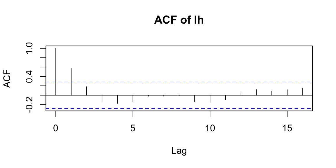
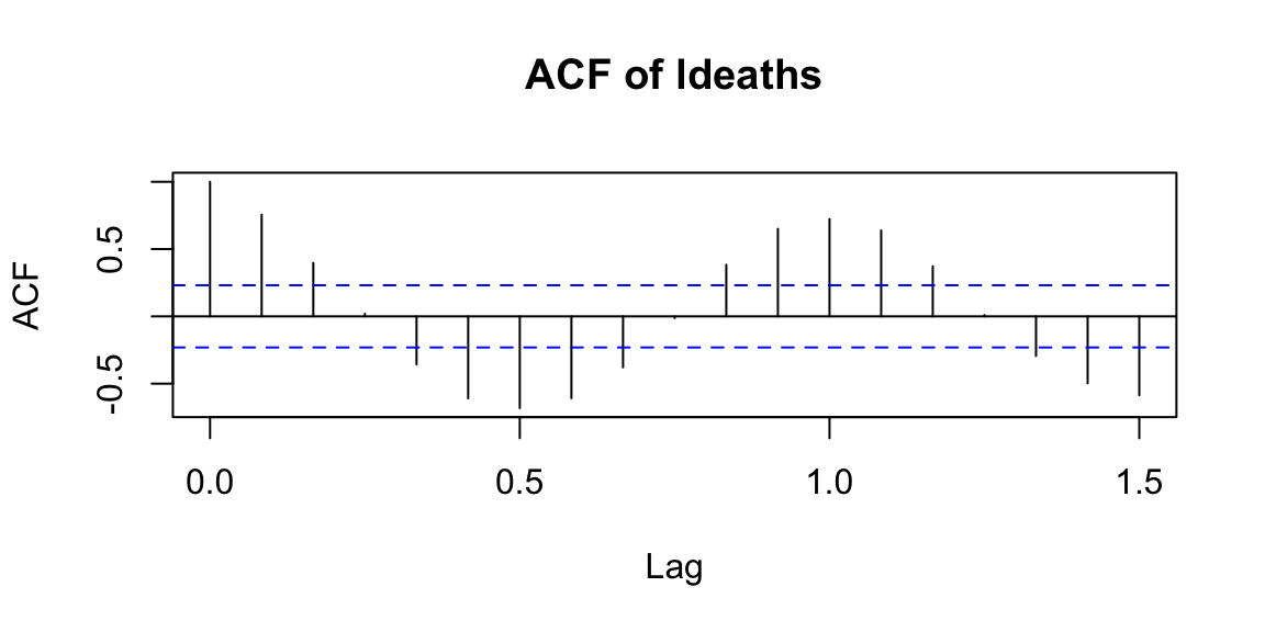
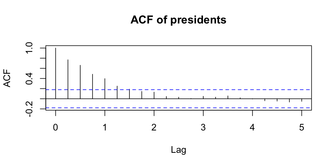
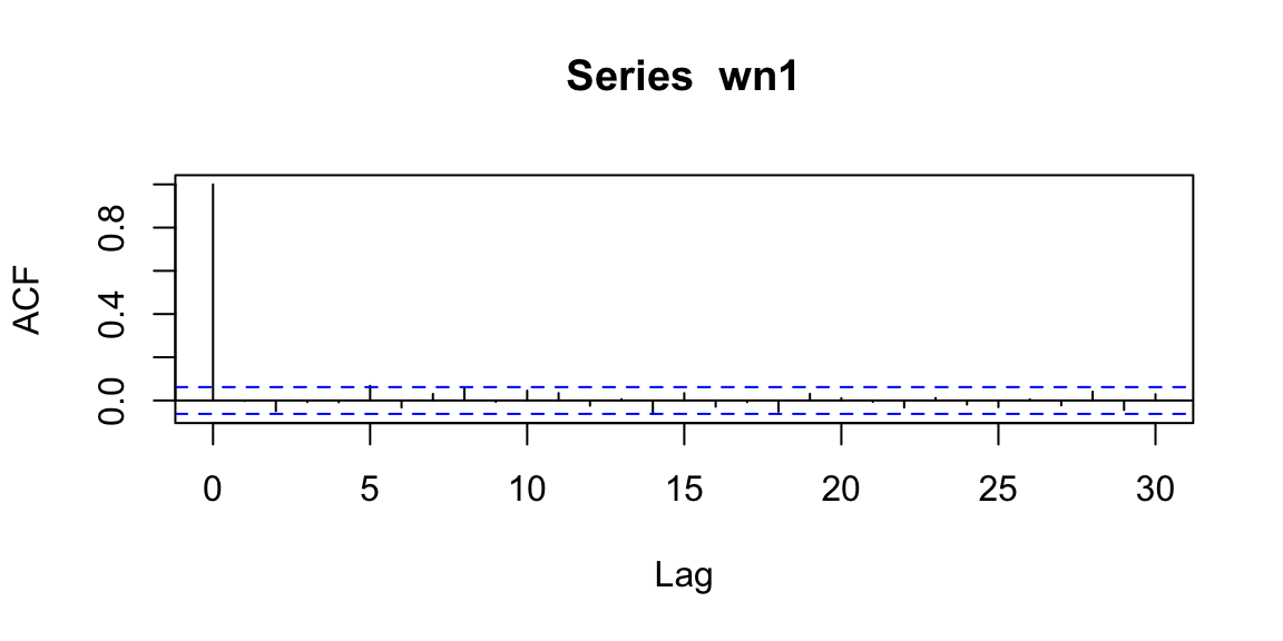
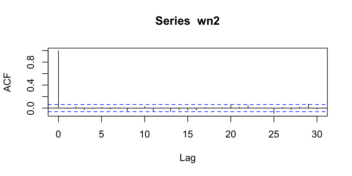
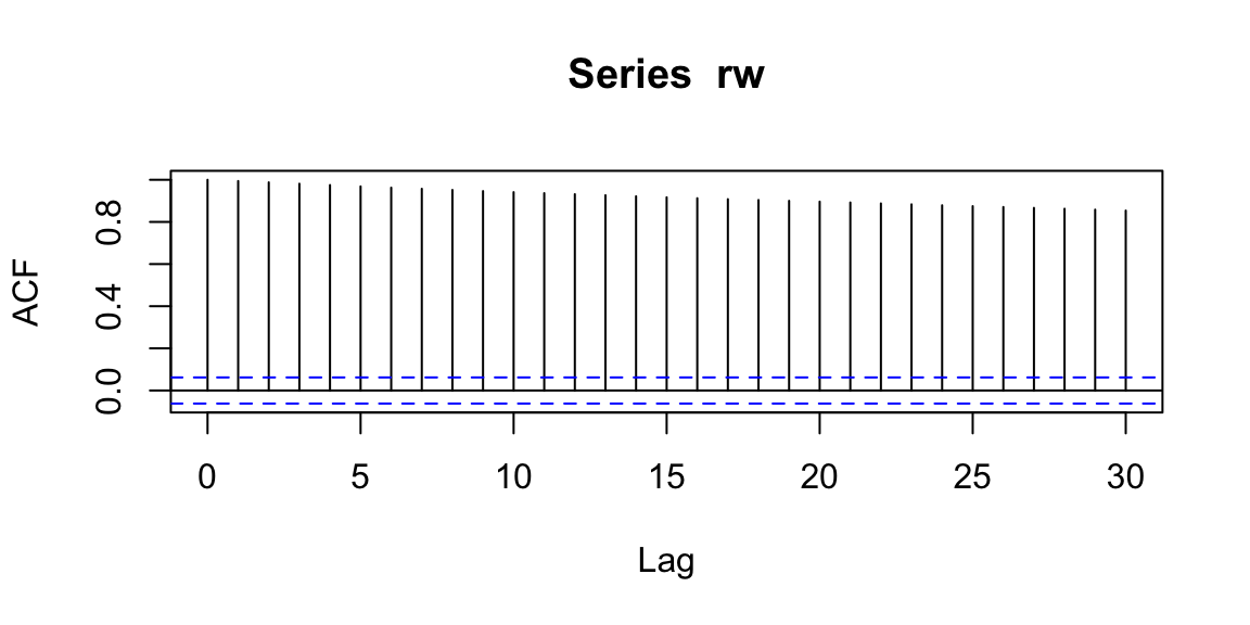
14.6.2 Autocorrelation function (ACF)
\[\rho_X(t_1,t_2)=\frac{\gamma_X(t_1,t_2)}{\sqrt{\gamma_X(t_1,t_1)\gamma_X(t_2,t_2)}}.\]
Properties:
- \(\rho_X(t_1,t_2)=\rho_X(t_2,t_1)\)
- \(-1 \leq \rho_X(t_1,t_2) \leq 1\)
Interpretation: ACF is an autocorrelation function which gives us values of autocorrelation of any series with its lagged (delayed) values. The ACF plot shows these values along with the confidence band. In simple terms, it describes how well the present value of the series is related with its past values. A time series can have components like trend, seasonality, cyclic and residual. ACF considers all these components while finding correlations.
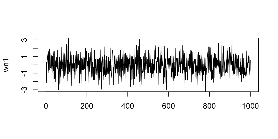
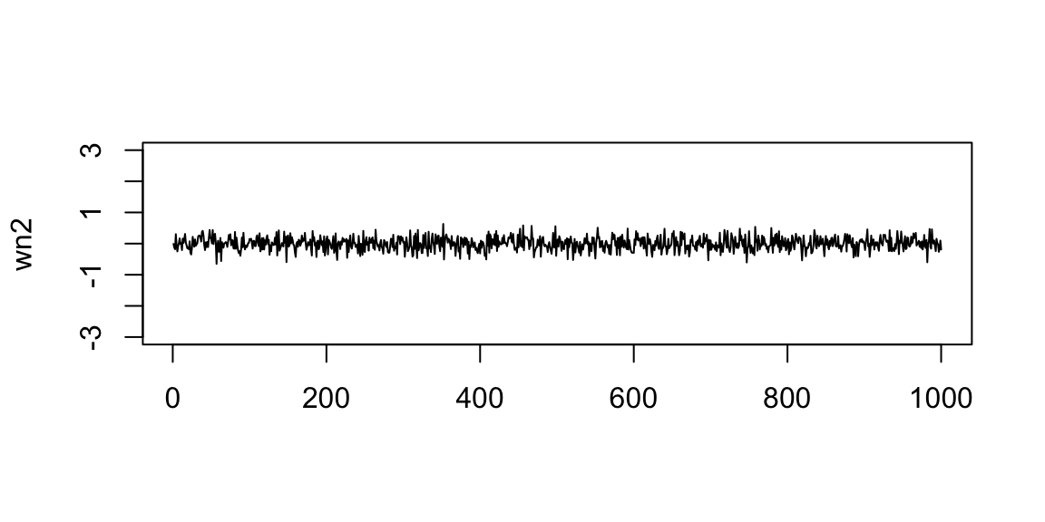
Examples:
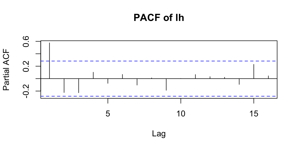
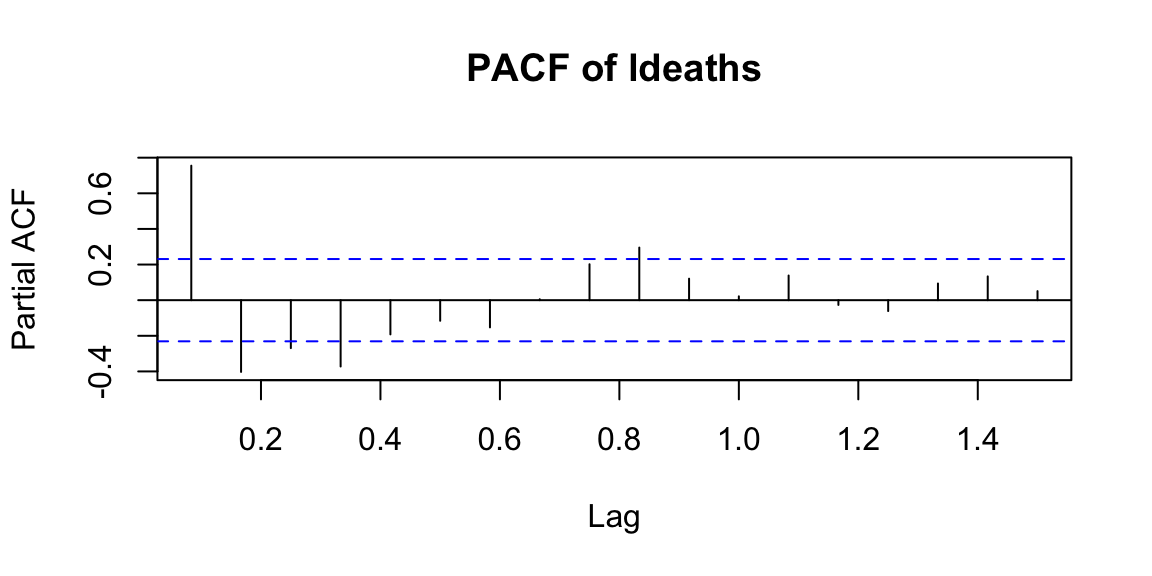
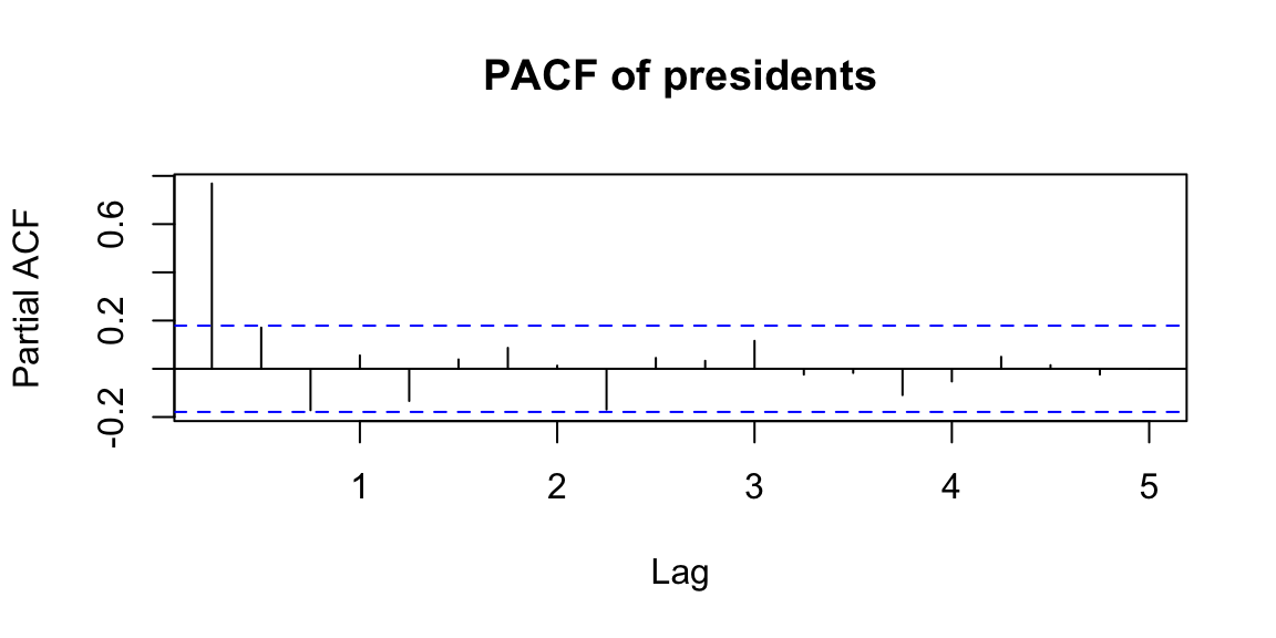
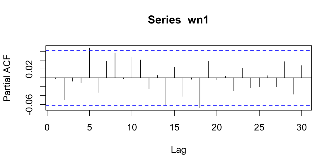
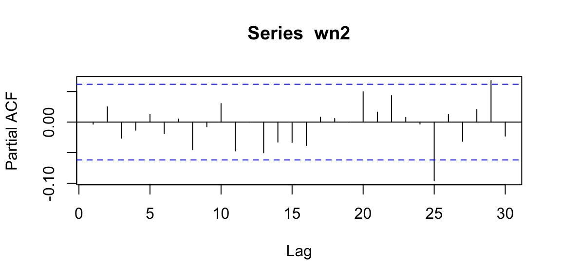
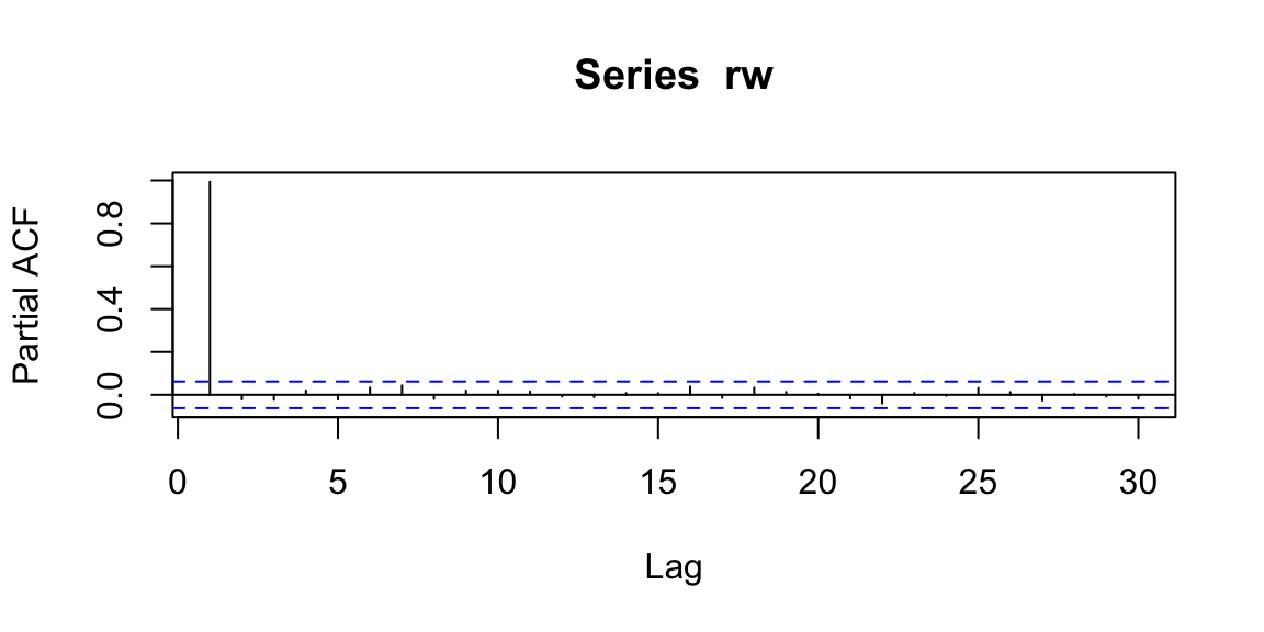
14.6.3 Partial autocorrelation function (PACF)
\[\phi_{kk}=Corr(X_t,X_{t-k} | X_{t-1},\ldots,X_{t-k+1})\] Interpretation: PACF is a partial autocorrelation function. PACF finds correlation conditional to past values.
Examples:
14.7 Classical decomposition models
Traditional methods consider the observed TS as a realization of the process \[X_t=f(T_t,S_t,Y_t),\] where
- \(T_t\) is the trend component: a trend exists when there is a long-term increase or decrease in the data.
- \(S_t\) is the seasonal component: a seasonal pattern occurs when a time series is affected by seasonal factors such as the time of the year or the day of the week.
- \(Y_t\) is the error component (usualy a standard white noise)
Models can be
- additive: \(X_t=T_t+S_t+Y_t\)
- multiplicative: \(X_t=T_t*S_t*Y_t\)
- mixtures: \(X_t=(T_t+S_t+Y_t)+(T_t*S_t*Y_t)\)
The estimated TS is \[\hat{Y_t}=X_t-T_t-S_t.\]
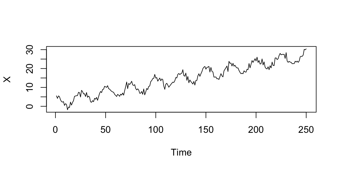
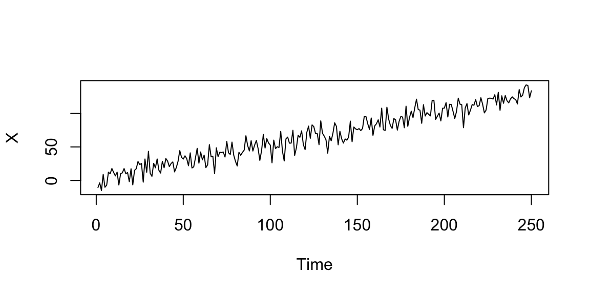
14.7.1 Classical decomposition models (trend component)
\[X_t=T_t+Y_t=(2+t/2)+Y_t, \quad Y_t \sim \mathcal{N}(0,10), \quad t=1,\ldots,250\]
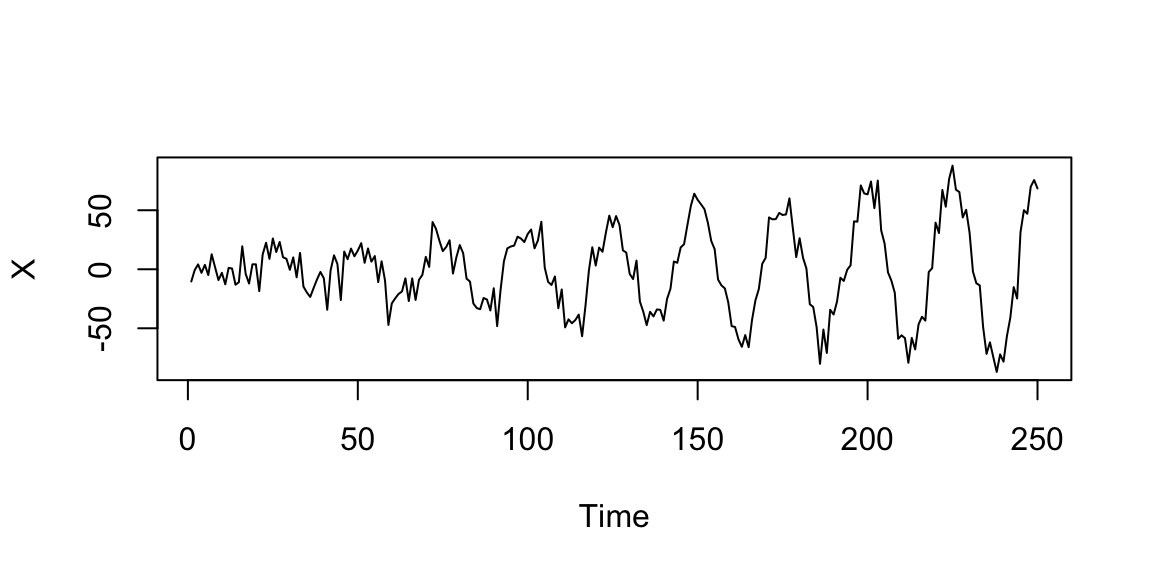
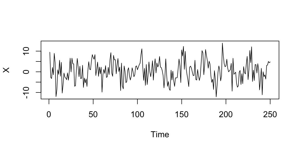
14.7.2 Classical decomposition models (seasonal component)
\[X_t=S_t+Y_t=3*\cos\left(\frac{2 \pi t}{25}\right)+Y_t, \quad Y_t \sim \mathcal{N}(0,4), \quad t=1,\ldots,250\]
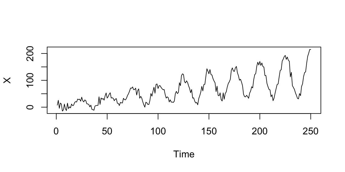
14.7.3 Classical decomposition models (additive model)
\[X_t=T_t+S_t+Y_t=(2+t/10)+3*\cos\left(\frac{2 \pi t}{25}\right)+Y_t, \quad Y_t \sim \mathcal{N}(0,1), \quad t=1,\ldots,250\]