6 Functions
Function examples:
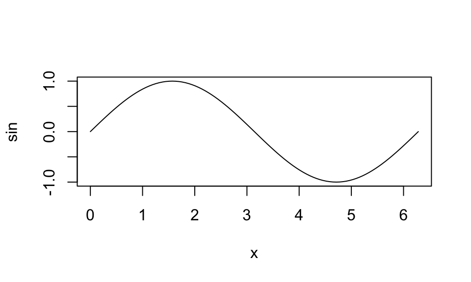
sin()integrate()plot()paste()
Typical input and output:
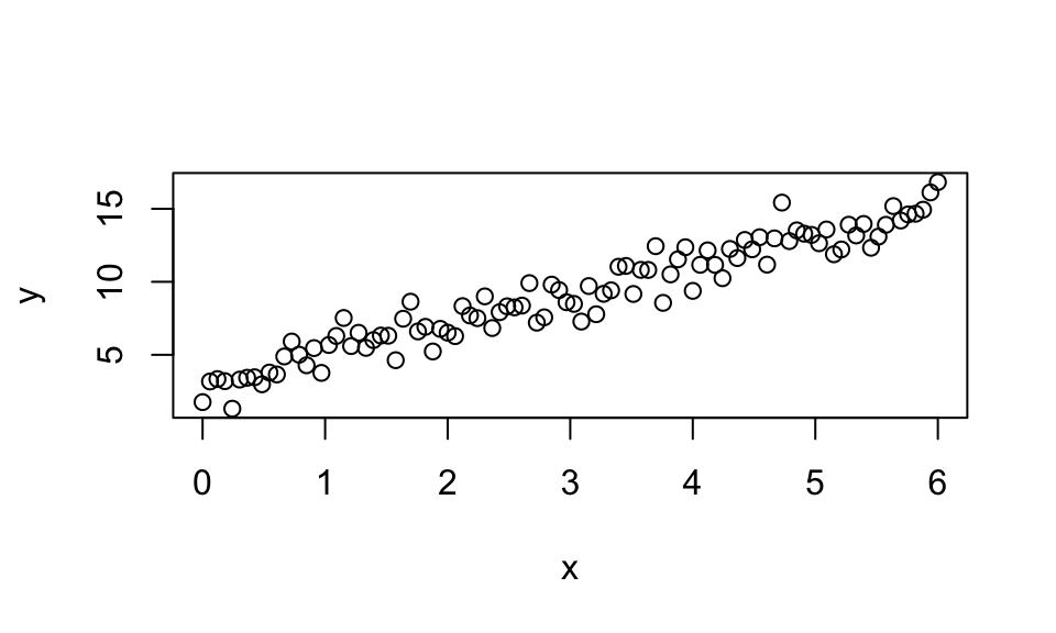
sin(): Input number, output number.integrate(): Input function and interval, output list (instead of a number!)plot(): Input vectors, output image.paste(): Input character objects, output one character object.
6.1 Simple Functions
- The above functions are built-in functions. However, it is simple to write your own functions:
6.4 Integrals and derivatives
6.6 Function source
If you write programs spanning more than a few lines it is convenient to write them in an editor.
A frequently used approach is to write your code in the editor and then paste blocks into R to run it.
Once the script is complete, the file is saved, and we can run it all by typing: